
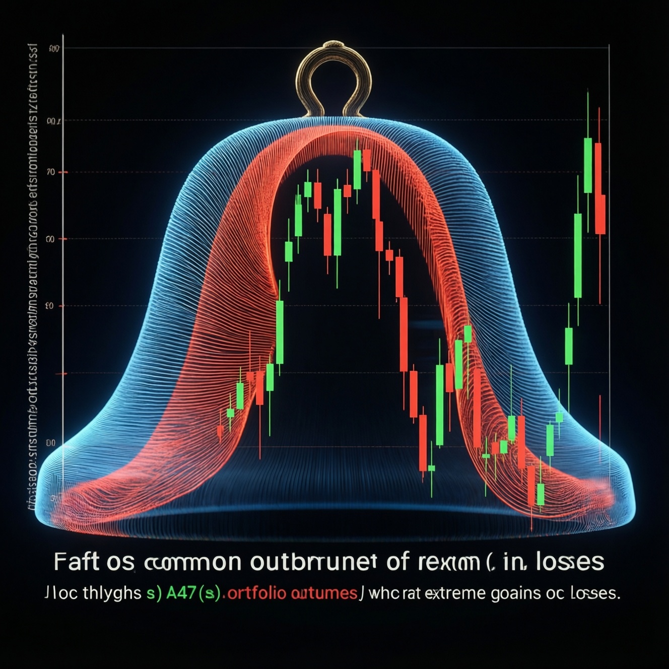
A return distribution is the spread of possible investment results over a chosen time horizon, showing what outcomes happen most often versus the rare, extreme gains or losses. It helps you interpret risk beyond average return, compare a stock return distribution to a portfolio return distribution, and choose models and position sizes that reflect real-world tails.
Core insights summary
- Most decisions should be driven by "typical" outcomes (center + dispersion), not by a single average.
- Median and mode often describe everyday results better than the mean when returns are skewed.
- Rare big hits (and crashes) live in the tails; they dominate long-run outcomes for many strategies.
- Normal assumptions simplify math but can understate tail risk; fat-tailed and mixture models are often more realistic.
- Return distribution analysis is only as good as its sampling window, data cleaning, and backtesting discipline.
- Practical portfolio design needs sizing rules and stress scenarios aligned with tail behavior.
Defining return distribution: metrics and typical shapes
The return distribution is the probability distribution of returns for an asset or strategy over a defined interval (daily, weekly, monthly, annual). In practice, you estimate it from historical data or simulations and use it to understand how frequently different outcomes occur.
Returns are usually defined as simple return R = (Pt − Pt−1)/Pt−1 or log return r = ln(Pt/Pt−1). Choose one and stick to it; mixing definitions silently distorts comparisons across instruments.
Common shapes include roughly symmetric "bell-like" distributions, skewed distributions (more frequent small losses with occasional large gains, or the reverse), and fat-tailed distributions where extreme outcomes occur more often than a normal model would suggest.
| Aspect | Most common outcomes (the "bulk") | Rare big hits (the "tails") | Why it matters in decisions |
|---|---|---|---|
| Where they sit | Near the center of the distribution | Far from the center, both positive and negative | Bulk drives day-to-day experience; tails drive survival and long-run compounding |
| Typical descriptors | Median, mode, interquartile range | Quantiles (e.g., left/right tail percentiles), max drawdown proxies | Center tells "what usually happens"; tails tell "what can break you or make you" |
| Model sensitivity | Often stable across reasonable model choices | Highly sensitive to assumptions and sample size | Tail estimates can swing widely; treat them as scenario ranges, not single truths |
| Operational impact | Helps set expectations, rebalancing bands, and risk budget usage | Drives stress tests, leverage limits, stop/hedge policies | Most processes fail in tails, not in the middle |
- Define the return horizon (daily vs monthly) before comparing distributions.
- Pick simple or log returns and keep it consistent across datasets.
- Separate "bulk" questions (typical range) from "tail" questions (extremes).
Where most outcomes lie: median, mode and dispersion

Most observations sit in the central mass of the distribution. To describe that "everyday zone," focus on robust measures of location and spread that don't get hijacked by a few extreme points.
- Median: the 50th percentile; a practical "typical outcome" when results are skewed.
- Mode: the most frequent return range; useful for understanding what you'll "see most days" in a trading strategy.
- Dispersion: use standard deviation for symmetric cases, but prefer IQR (75th-25th percentile) when tails are heavy.
- Asymmetry check: compare mean vs median; a big gap hints that rare events are pulling the average.
- Time scaling caution: the "monthly distribution" is not just the daily distribution multiplied by a constant; compounding and autocorrelation can change shape.
- Portfolio layer: in a portfolio return distribution, correlations reshape the bulk-diversification usually tightens the center even if tails remain.
- Use median + IQR as a default summary alongside mean + stdev.
- Check whether mean and median differ materially before trusting "average return."
- Recompute summaries per regime (e.g., calm vs volatile months) rather than one blended number.
Rare big hits: tail behavior, skewness and kurtosis
Tails describe extreme outcomes. Positive tail events are "rare big hits"; negative tail events are crashes, gaps, and liquidity shocks. Skewness indicates whether outsized outcomes tend to be on the upside or downside; kurtosis reflects tail heaviness (how often extremes appear).
- Single-name equity selection: a stock return distribution can be right-skewed if a few breakout moves dominate multi-year performance; missing them can erase the strategy's edge.
- Options selling / carry trades: often show small frequent gains with occasional sharp losses (left-tail risk); the bulk looks safe until a tail arrives.
- Trend-following: can exhibit "crisis alpha" behavior where right-tail outcomes occur during stress; the tail is a feature, not noise.
- Illiquid assets: returns can look artificially smooth, then jump (stale pricing); tails may be hidden until repricing events.
- Thailand context (THB exposure): FX-linked holdings can add tail risk when local currency moves coincide with global risk-off days.
- Identify whether your strategy relies on a few rare outsized winners (right tail).
- Stress the left tail explicitly if you harvest small premia (carry, short vol).
- Assume tails cluster during market stress; don't treat extremes as independent.
Modeling choices: normal, fat-tailed and mixture models
Models are simplifications for decision-making. The key is to match the model to the question: describing the bulk, estimating tail risk, or generating scenarios for stress tests.
Common modeling options and when they fit
- Normal model: convenient baseline for symmetric bulk behavior; often underestimates extremes if tails are heavy.
- Student-t (fat-tailed): keeps a single distribution but allows more extreme outcomes; useful when "normal" misses observed tail frequency.
- Mixture models (regimes): combine multiple states (e.g., calm + stressed) to capture volatility clustering and shape shifts.
- Empirical / bootstrap: resample observed returns; good for transparency, but inherits history's gaps and biases.
Practical limitations to keep in mind
- Parameter instability: tail parameters are fragile; small data changes can swing results.
- Model risk: different models can agree in the center and disagree wildly in the tails.
- Hidden dependence: correlations rise in stress; modeling assets independently can understate portfolio tail risk.
- Overfitting: extra flexibility (mixtures) can fit noise; prefer models that generalize out-of-sample.
- Use a normal model only as a baseline, not as a tail-risk engine.
- Compare at least one fat-tailed or regime-based alternative when decisions depend on extremes.
- Document which decisions use which model (bulk vs tails) to avoid "model drift."
Measuring reality: sampling limits, outliers and backtesting
Estimating an investment return distribution from data is less about fancy math and more about avoiding measurement traps that quietly reshape the distribution.
- Wrong horizon: mixing daily and monthly intuition leads to misread risk; always label the time step.
- Survivorship bias: analyzing only current constituents can make the distribution look safer and more profitable than it was.
- Outlier mishandling: deleting extremes "because they look wrong" can remove the very tail events you must manage.
- Overlapping windows: rolling returns create dependence; treat them as smoothed views, not independent samples.
- In-sample tuning: calibrating thresholds to past extremes often fails out-of-sample; keep a clean separation for backtesting.
- Write down your sampling choices: period, universe, filters, and corporate action handling.
- Flag and investigate outliers, but avoid auto-deleting them without a documented rule.
- Run out-of-sample checks whenever you tune a strategy using distributional features.
Practical consequences: sizing, diversification and stress scenarios
Distribution thinking becomes actionable when it changes how you size positions, combine assets, and plan for tail scenarios. A portfolio can have a tight "bulk" yet still carry dangerous left-tail exposure if constituents become correlated during stress.
Mini-scenarios (use cases you can copy)
- Concentrated stock bet (SET-listed equity): if your stock return distribution is right-skewed, cap position size so one left-tail event cannot dominate the portfolio, while still letting right-tail winners matter.
- Income strategy (short volatility / option selling): treat small frequent gains as bulk; size primarily against left-tail scenarios (gap moves, volatility spikes), not against average monthly return.
- Balanced multi-asset book: build diversification for the center (lower everyday volatility), then add explicit tail hedges or reduce leverage to survive correlation spikes.
Simple workflow (pseudo-steps) for return distribution analysis
- Define: horizon, return type (simple or log), and the exact universe.
- Summarize bulk: median, mode (binned), IQR; compare against mean and stdev.
- Probe tails: inspect left/right quantiles; run stress scenarios that represent plausible tail moves.
- Model-check: compare normal vs fat-tailed vs regime/mixture outputs; note where tails diverge.
- Decide: set sizing and limits based on tail tolerance; set rebalancing rules based on bulk behavior.
- Translate distribution outputs into explicit limits (max position, max leverage, max drawdown tolerance).
- Use diversification to stabilize the bulk, then address tails with scenarios and constraints.
- Revisit assumptions when regimes change (volatility, correlation, liquidity).
- Did I summarize both the bulk (median/IQR) and tails (quantiles/stress scenarios)?
- Did I separate decisions that rely on typical outcomes from decisions that must survive extremes?
- Did I test at least one fat-tailed or regime alternative to a normal assumption?
- Did I document horizon, universe, and outlier rules so results are reproducible?
Clarifying common doubts about return behavior
Is the mean return the best "typical" outcome?
Not when returns are skewed or fat-tailed. The mean can be pulled by rare big hits (or crashes), so median and mode often describe day-to-day outcomes better.
How is an investment return distribution different from volatility?
Volatility is one summary of spread, typically tied to standard deviation. A full distribution also shows asymmetry and tails, which can dominate real risk.
Why can a portfolio return distribution look safer than each asset alone?
Diversification can tighten the center when assets aren't perfectly correlated. In stress, correlations can rise, so the tails may not improve as much as the bulk.
Do rare big hits matter if they happen infrequently?
Yes, because a small number of extreme outcomes can drive long-run results and determine survival. This is especially true for strategies with asymmetric payoff profiles.
Is a normal model ever acceptable for return distributions?
It can be a useful baseline for the bulk when data looks roughly symmetric. For tail-sensitive decisions (leverage, risk limits), compare it with fat-tailed or regime models.
What is the fastest way to start return distribution analysis?
Define the horizon, compute consistent returns, then summarize median/IQR and tail quantiles. Use the same pipeline across assets to compare a stock return distribution and a broader portfolio.